Free-surface wave
The Problem
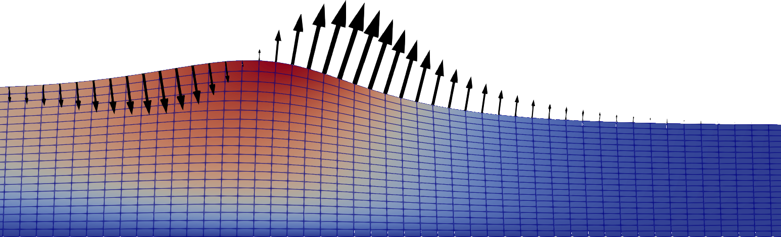
In this example we will simulate a simple 2D free-surface wave in a container with symmetry conditions on both sides. We start the simulation with a sinusoidal displacement of the fluid but with the fluid being at rest. Due to the presence of gravity the wave will then start moving forward. To make the simulation setup as simple as possible we will assume a highly viscous fluid (\(\nu = 10^{-3} \, \text{m}^2 / \text{s}\)).
Running the simulation
The case can be found in examples/free-surface-wave/. To run the simulation run
blockMesh
foamRun
to first create the mesh and then to start the simulation. Use
paraFoamto visualize the result.
The Allclean script can be used to remove the simulation results.
Solver setup
For the solver we will choose the incompressibleFluid solver (the equivalent of simpleFoam and pimpleFoam in earlier OpenFOAM versions):
// from system/controlDict
application     foamRun;
solver          incompressibleFluid;
This solver solves the pressure field and velocity field for an incompressible fluid of constant material properties. To include the effect of gravitational acceleration we will use the fvModel called buoyancyForce:
// from constant/fvModels
buoyancyForce
{
    type        buoyancyForce;
}
This will add the gravitational acceleration as a source term to the momentum equation. The acceleration vector is specifie as a field in constant/g.
Since we are planning on using an implicit treatment of the free surface velocity, we need to set the moveMeshOuterCorrectors to true in the solution algorithm (the opposite would be true if we want to use an explicit treatment). It is also recommended to set correctPhi to true for moving meshes:
// from system/fvSolution
PIMPLE
{
    moveMeshOuterCorrectors  true;
    correctPhi               true;
    //...
}
Dynamic Mesh setup
To enable mesh movement for the simulation, we need a file called dynamicMeshDict inside the constant/ directory. Here we must choose a motionSolver that handles the mesh movement. In principle, we have two options: The builtin velocityLaplacian or the explicitImplicitVelocityLaplacian that is introduced with this library. The builtin velocityLaplacian should be used for a purely explicit time integration of the mesh velocity and the explicitImplicitVelocityLaplacian for any other case. We will choose the explicitImplicitVelocityLaplacian for this example:
// from constant/dynamicMeshDict
mover
{
    type motionSolver;

    motionSolver    explicitImplicitVelocityLaplacian;
    theta           1;
    diffusivity     uniform;
}
theta set to 1 means that we treat the mesh velocity fully implicitely.
The motionSolver will instanciate the field pointMotionU which holds the values for the mesh velocity. On the free surface (in the example the patch is called freeSurface) we use the kinematicSurfaceVelocity boundary condition which is introduced with this library:
// from 0/pointMotionU
freeSurface
{
    type                        kinematicSurfaceVelocity;
    linearUpwindBlendingFactor  0.97;
    laplaceSmoothing            true;
    value                       $internalField;
}
This boundary condition will set the mesh velocity equal to the surface-normal component of the velocity field.
Boundary conditions for \(p\) and \(U\)
For the pressure field we will assume assume a constant value on the free surface patch. For the other boundaries we will use the fixedFluxPressure boundary condition. This boundary condition is used as due to the gravitational acceleration we can not use a zero gradient condition. The fixedFluxPressure boundary condition is exactly made for this scenario.
For the velocity field we will use a zeroGradient boundary condition. This corresponds to the assumption of no shear stress on the surface.